Measuring Egalitarian Attitudes Using Twitter

09 Aug 2019

The Research Question

Social egalitarianism, the respect for all persons regardless of their ascriptive characteristics (religion, ethnicity, language, race, sex, sexual orientation, or nationality), is intimately tied with the Western liberal political tradition.¹ What is the spatial mapping of support for social egalitarian values? In a project with John Gerring and Steven Wilson, we attempt to answer this question using Twitter data.

Natural Language Processing (NLP) tools have been applied to a variety of political questions using tweets as source material (see, e.g. Halberstam & Knight or Barberá for a tiny sampling of the fascinating work out there on this topic).

This previous work has provided some important insights and advanced our understanding of various political processes. However, none of these previous approaches is sufficient to identifying egalitarian tweets. Our topic is abstract, broad, and infrequently discussed directly on Twitter.

A classification problem of this kind requires a supervised model, in turn requiring hand coded data for training and validation. Here again, our research question is problematic. Given the rarity of the topic, finding a sufficient number of relevant tweets from a random sample poses a significant challenge and finding them based on a keyword search imposes researcher priors we seek to avoid. Finally, because the relative classes are so unbalanced, the amount of training data required is an order of magnitude higher than a case with balanced classes. In short, we want to train a machine to identify a needle in a haystack, but we must first find many needles ourselves to train the machine.

Our Approach

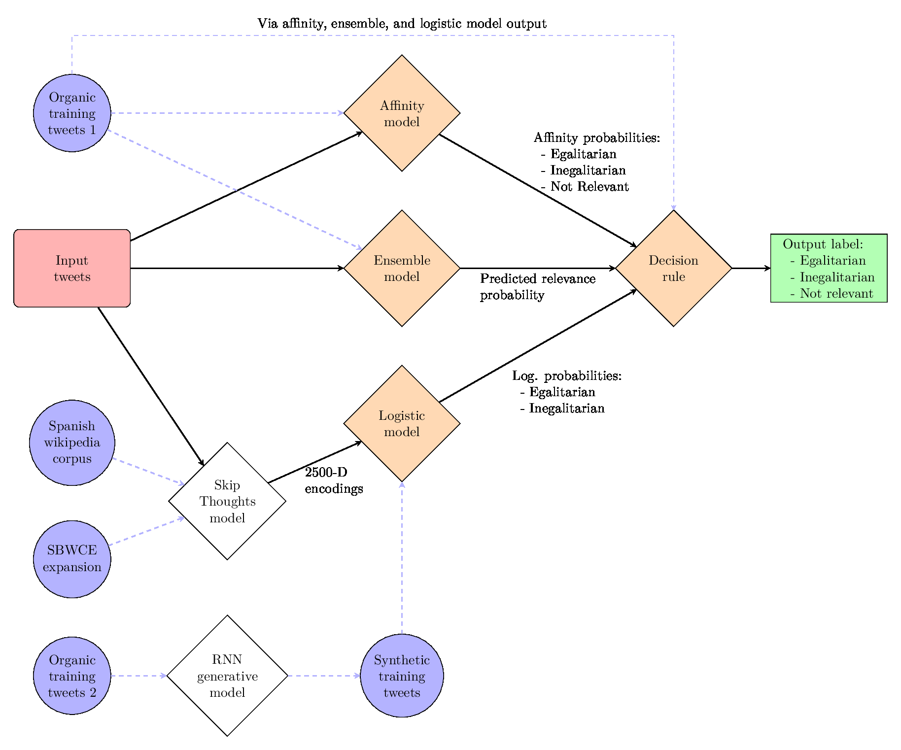
To overcome these difficulties, we design the following novel hybrid model:

In the final classification, input tweets (red rectangle) are fed into three models and the predictions of each are adjudicated by a decision rule model to produce an output label (green rectangle) of egalitarian, inegalitarian, or not relevant. All diamonds represent models, with orange fill corresponding to supervised models and white fill corresponding to unsupervised models. Input data is represented in the figure by blue circles. I will outline here the bottom and right-hand portions of this model.

First note that a selection of approximately 8,000 hand-coded tweets is first divided into three parts: one that is used to train the affinity and ensemble models using bag-of-words encodings, a second that is used to train the decision rule (after being fed through the pre-trained affinity, ensemble, and logistic models), and a third, smaller, test set held out for validation.

Logistic Model

The logistic model takes as inputs tweets that have been encoded using a sentence-level skip-gram model. The encodings are 2400-dimensional. The logistic model itself is a plain-vanilla non-linear classifier trained using synthetic training tweets from a combination of generative recurrent neural nets. The model uses an l2 penalty and regularization factor of 1/5 selected through a grid search algorithm maximizing classification accuracy.

Generative RNNs

We first divide the general egalitarian topic into subtopics covering each of the constituent parts: women’s rights, gay rights, civil rights and liberties, immigration, and religious freedom. We further break those into positive and negative sentiment for a total of ten subtopics and train a separate RNN for each. To collect training data for these models, we identify Twitter accounts that post exclusively on the given subtopic. Finding accounts that tweet on a single one of these topics (often organizations dedicated to that topic) is an easy task for the positive aspect, but very challenging for the negative. As a result, we combine anti-gay rights, anti-civil rights and liberties, anti-immigration, and anti-religious freedom into a single model (keeping anti-women’s rights as a distinct model), reducing the total to seven generative models. Downloading the tweets from these accounts yields approximate 20,000 tweets for each of the seven models. These tweets are referred to as “Organic Training Tweets 2”

The RNN model itself is a plain-vanilla RNN working at the character level. It is provided by Justin Johnson and is available at https://github.com/jcjohnson/torch-rnn. The model is written using the Lua and Torch. Each model has 4 layers of 512 neurons and a 0.3 dropout between each layer. The models are trained in batches of 100 tweets and sequence lengths of 140 characters. Because tweets may contain line breaks, each is padded with a special end of sequence tag. Thus, even though the model is fed sequences of 140 characters, it will learn to generate texts of lengths distributed the same was as real tweets, accommodating both the bulk of tweets less than 140 characters as well as those that follow the new longer limit of 280 characters. Model training is done in chunks of 10 epochs and then generative output is tested for plausibility. Once tweets generated at a medium “temperature” (discussed in greater detail below) are indistinguishable from real tweets, training is stopped.

In its generative mode, the model takes a “temperature” parameter. This controls the sampling probability of the final softmax layer in the model. Ranging from 0 to 1, higher temperatures correspond to noisier (less likely) characters being chosen by the model.

Experimentation demonstrated that very low temperatures produced unusable results (long repetitions of a “hashtag” label, for example). Thus for each of the seven generative models, smaller samples were taken at every 0.1 for temperatures ranging from 0.2 to 1.0. The results were examined and plausible ranges for each model established. The goal was to generate 10,000 tweets for each model. The better performing the model (as judged by preliminary samples), the more weight was given to higher temperature tweets to maximize the diversity of training data generated. Thus, for example, the target 10,000 pro-women’s rights tweets was generated with 25% at 1.0, 25% at 0.9 and 10% for each tenth from 0.4 to 0.8.

The output is nearly 70,000 tweets constituting the “Synthetic Training Tweets.”

Sentence level Skip-Gram (Skip-Thoughts)

This model was first described by Kiros et al. It follows a typical skip-gram architecture, but instead of taking words as inputs, it takes sentences. Kiros et al. produce a trained model for English. In order to train a Spanish-language version, we feed it a dump of Spanish Wikipedia from March 20, 2018 and use the Tensorflow implementation of the model provided by Chris Shallue.

Sentences are processed in the following way. First, they are tokenized using the NLTK Spanish tokenizer. These tokens are then converted to a numerical vector using a simple dictionary mapping using the top 20,000 words and are padded to a target length of 128 (the batch size). Words outside the top 20,000 are assigned a special value for “unknown word”.

The model relies on gated recurrent unit (GRU) cells and defaults to 620 cells. The model is trained for 500,000 steps with a decay of 0.5.

After training the original model, we expand the vocabulary, again following the procedure described in Kiros et al (2015). The procedue is train a linear model to learn mappings between the embeddings in our trained skip-thoughts model to a pre-trained word2vec model. In this case, we use a Spanish language word2vec model from the Cristian Cardellino’s Spanish Billion Words Corpus and Embeddings project. The expansion words by using a linear model to map the embeddings of one model onto the other, thus allowing the skip thoughts model to move from an original vocabulary of 20,000 words to over 1.2 million.

Decision Model

The decision model is a random forest that takes as input the predicted class probabilities from the affinity and logistic models as well as the predicted relevance from the ensemble model. It outputs a class prediction. This model is trained using the predictions generated by the three models when Organic Training Set 1 are fed through them.

The forest parameters are: max depth 10, max features 5, number estimators 25.

Results and Next Steps

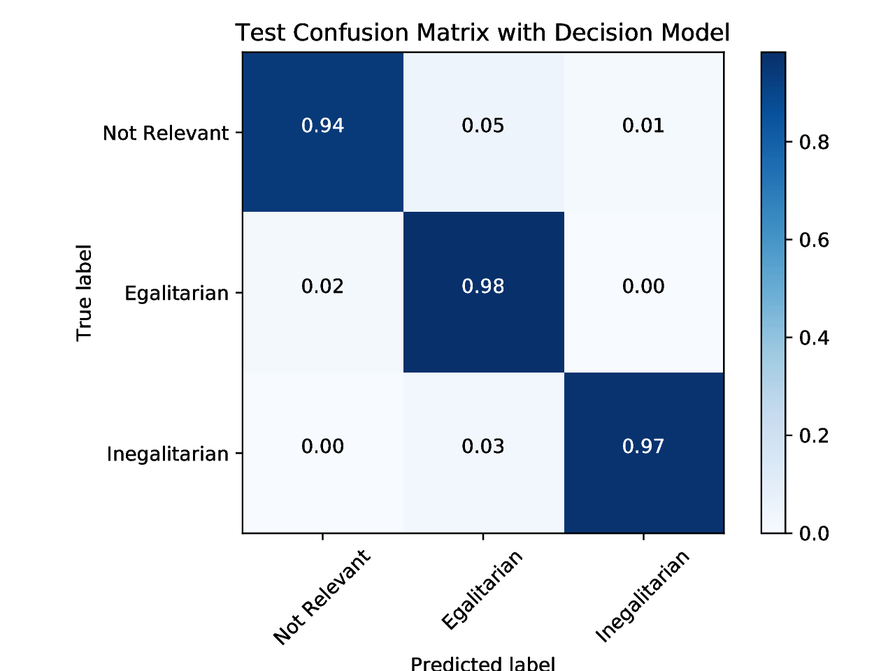
Does this approach work? In a word, yes. The following confusion matrix shows the results from a validation on the withheld hand-coded tweets:

The results are very encouraging! We’ve labeled 94% of the not relevant tweets correctly and 98% and 97% of the egalitarian and inegalitarian tweets, respectively! The classifier is imperfect — we have both false positives and false negatives — but the rates are very low considering that original task.

It’s worth noting that when a tweet is mislabeled, it is much more likely to be put into the egalitarian than the inegalitarian category. This suggests that we could take a closer look at each of the model components and try to boost the performance of the ones that are best at labeling inegalitarian tweets. Since all model parameters have been tested and maximized already, the best option here is probably to increase the available training data.

For further validation we’ll also want to take a look at some of the model output for a new sample of data and make sure that a human finds the predictions plausible!

As I alluded to at the start of this post, once we have finalized the classifier, we want to use the data to explore larger questions in political science. Notably, we’re interested in how these values map geographically.

As we continue to look for ways to improve model performance, we welcome any feedback or suggestions!

Notes